| Prev: Installation | Current: SQL Queries | Next: – |

This is a continuation to the basics of database for non-programmers. We will only be discussing SQL selection. We will not be discussing any DDL queries, nor any inserts or updates type DMLs – just DQL (Data Query language). This is going to be a long one, so brace for impact.
Beginning
Since we are working with MySQL, let’s first see how MySQL defines their Select statement format.
SELECT
    [ALL | DISTINCT | DISTINCTROW ]
    [HIGH_PRIORITY]
    [STRAIGHT_JOIN]
    [SQL_SMALL_RESULT] [SQL_BIG_RESULT] [SQL_BUFFER_RESULT]
    [SQL_NO_CACHE] [SQL_CALC_FOUND_ROWS]
    select_expr [, select_expr] ...
    [into_option]
    [FROM table_references
      [PARTITION partition_list]]
    [WHERE where_condition]
    [GROUP BY {col_name | expr | position}, ... [WITH ROLLUP]]
    [HAVING where_condition]
    [WINDOW window_name AS (window_spec)
        [, window_name AS (window_spec)] ...]
    [ORDER BY {col_name | expr | position}
      [ASC | DESC], ... [WITH ROLLUP]]
    [LIMIT {[offset,] row_count | row_count OFFSET offset}]
    [into_option]
    [FOR {UPDATE | SHARE}
        [OF tbl_name [, tbl_name] ...]
        [NOWAIT | SKIP LOCKED]
      | LOCK IN SHARE MODE]
    [into_option]

into_option: {
    INTO OUTFILE 'file_name'
        [CHARACTER SET charset_name]
        export_options
  | INTO DUMPFILE 'file_name'
  | INTO var_name [, var_name] ...
}
Overwhelming stuff, right? We will break it up in small chunks and tackle a lot of these as we go in this blog. We will use the database that we imported to test out all the features.
Entity Relationship Diagram
Before we start, we will take a step back and look at something called Entity Relationship (ER) diagram. Briefly, ER diagram shows the relationship between different objects (entities) in the database. In this case you can consider tables as entities. It can also define the attributes for these entities. Let’s see the auto generated ERD for the database we loaded.
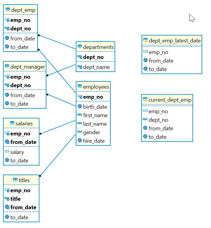
The items in yellow background indicate table names. Attributes in bold are the primary keys. We see that employees table is being used by dept_manager, salaries and titles. Same with departments. It is referred to by dept_emp and dept_manager. On the other hand, dept_emp_latest_date and current_dept_emp are not related to any other tables.
Basic Selection from tables
We will start with a simple query. We will query everything in departments table.
select *
  from employees.departments d
;
| dept_no | dept_name |
|---|---|
| d009 | Customer Service |
| d005 | Development |
| d002 | Finance |
| d003 | Human Resources |
| d001 | Marketing |
| d004 | Production |
| d006 | Quality Management |
| d008 | Research |
| d007 | Sales |
We could have also specified all the column names instead of ‘*’. Of course we can also selectively specify the column names. The query above is equivalent to following query,
select dept_no, dept_name
  from employees.departments d
;
However, imagine that you do not want to select all records in the table. We could easily set a limit to the count of records we fetch. We use the LIMIT keyword as seen below to limit results.
select dept_no, dept_name
  from employees.departments d
 limit 5
;
| dept_no | dept_name |
|---|---|
| d009 | Customer Service |
| d005 | Development |
| d002 | Finance |
| d003 | Human Resources |
| d001 | Marketing |
That’s all good, but I need to sort by dept_no. How do I do that? SQL provides ORDER BY clause to help you in that.
select dept_no, dept_name
  from employees.departments d
 order by dept_no
 limit 5
;
| dept_no | dept_name |
|---|---|
| d001 | Marketing |
| d002 | Finance |
| d003 | Human Resources |
| d004 | Production |
| d005 | Development |
If you run a select on employee.titles, you will see a lot of different titles. I want to find all the unique titles that can be assigned to an employee. SQL provides the DISTINCT keyword. We use it to find unique values from a column.
select distinct title as "ALL TITLES"
  from employees.titles t
 order by 1
;
| ALL TITLES |
|---|
| Assistant Engineer |
| Engineer |
| Manager |
| Senior Engineer |
| Senior Staff |
| Staff |
| Technique Leader |
As you can see, we are using two new things in the query above too. The first one we have is as “ALL TITLES”. This is known as alias. In this case we are naming the output column to ALL TITLES. The other thing that we see is in ORDER BY clause. Here we have number 1 instead of a column name. We can always specify column position in ORDER BY clause. This is not a recommended practice since this has to be changed as soon as the selection criteria is changed.
Conditionals
We will discuss the following keywords in this section.
- WHERE – adds a specific condition to search on a column
- =, >, <, >=, <= – comparison operators
- AND – used with where to specify additional conditions to add to existing
- OR – used to specify a either/ or condition with existing
- NOT – this is used to negate a condition
- IN – takes an array of values to search for
- BETWEEN – takes two values and find all records matching within them
- LIKE – wildcard search
We will take some examples and query them. This will give a good idea of how each clause works. I will LIMIT all resultset to top 5, but you should see a lot more records when running the queries.
Q 1. Find the employee with employee ID = 10290.
select * from employees.employees e
 where emp_no = 10290
;
| emp_no | birth_date | first_name | last_name | gender | hire_date |
|---|---|---|---|---|---|
| 10,290 | 1957-05-29 | Yongmao | Pleszkun | M | 1991-09-18 |
Q 2. Find all employees with first name as Mary and employed after 1st January, 1998.
select * from employees.employees e
 where first_name = 'Mary'
   and hire_date > '1998-01-01'
;
| emp_no | birth_date | first_name | last_name | gender | hire_date |
|---|---|---|---|---|---|
| 20,819 | 1955-12-28 | Mary | Ritcey | M | 1998-07-06 |
| 256,230 | 1962-03-09 | Mary | Peha | M | 1998-07-31 |
| 486,829 | 1953-10-11 | Mary | Facello | M | 1998-02-13 |
Here we have used the > than operator. This is a very flexible operator and works on Numerics, Strings and like in this case Dates. We also used AND operator.
Q 3. Find all female employees who were either hired before or equal to 1st January, 1985 or were hired after or equals 1st of January, 2000 order by hire_date in descending order.
select * from employees.employees e
 where gender = 'F'
  and (hire_date >= '2000-01-01'
   or hire_date <= '1985-01-01')
 order by hire_date desc
;
| emp_no | birth_date | first_name | last_name | gender | hire_date |
|---|---|---|---|---|---|
| 499,553 | 1954-05-06 | Hideyuki | Delgrande | F | 2000-01-22 |
| 222,965 | 1959-08-07 | Volkmar | Perko | F | 2000-01-13 |
| 422,990 | 1953-04-09 | Jaana | Verspoor | F | 2000-01-11 |
| 205,048 | 1960-09-12 | Ennio | Alblas | F | 2000-01-06 |
| 226,633 | 1958-06-10 | Xuejun | Benzmuller | F | 2000-01-04 |
| 60,134 | 1964-04-21 | Seshu | Rathonyi | F | 2000-01-02 |
| 72,329 | 1953-02-09 | Randi | Luit | F | 2000-01-02 |
| 110,183 | 1953-06-24 | Shirish | Ossenbruggen | F | 1985-01-01 |
| 110,303 | 1956-06-08 | Krassimir | Wegerle | F | 1985-01-01 |
| 110,725 | 1961-03-14 | Peternela | Onuegbe | F | 1985-01-01 |
| 111,692 | 1954-10-05 | Tonny | Butterworth | F | 1985-01-01 |
We introduced some new things in the query above. First we put braces around the hire_dates. This will always be evaluated first (similar to how it is in algebra). We have added a DESC clause to ordering. Default ordering is ASC 9or ascending). We also introduced OR clause in the statement.
Q 4. Select all employees with ID: 10001, 10002, 10003, but do not show any female employees.
select * from employees.employees e
 where emp_no in (10001, 10002, 10003)
   and gender != 'F'
;
| emp_no | birth_date | first_name | last_name | gender | hire_date |
|---|---|---|---|---|---|
| 10,001 | 1953-09-02 | Georgi | Facello | M | 1986-06-26 |
| 10,003 | 1959-12-03 | Parto | Bamford | M | 1986-08-28 |
In this case, employee 10002 is female, so even though it would have been selected,
Q 5. Select all employees hired between 1st of May, 1995 and 31st of May, 1995 limit to 5 employees.
select * from employees.employees e
 where hire_date between '1995-05-01' and '1995-05-31'
 limit 5
;
| emp_no | birth_date | first_name | last_name | gender | hire_date |
|---|---|---|---|---|---|
| 10,239 | 1955-03-31 | Nikolaos | Llado | F | 1995-05-08 |
| 11,049 | 1963-02-12 | Gift | Apsitis | F | 1995-05-12 |
| 11,055 | 1956-08-10 | Shaleah | Neiman | M | 1995-05-25 |
| 11,408 | 1961-01-13 | Shahab | Serot | F | 1995-05-28 |
| 12,042 | 1959-08-02 | Torsten | Swan | F | 1995-05-19 |
Here we introduced BETWEEN. This is used to select data between the minimum and maximum values specified.
Wildcards
Before we start working on LIKE, let us talk about wildcards. SQLs support two different characters that are used for wildcards.
- ? – This is used for matching a single character
- % – This is used for matching multiple characters
A wildcard can be used in front or end or both sides of a search string. Whenever a wildcard is used, search with equals (=) operator is not possible. We will be using LIKE search for wildcards. Now let’s try an example.
Q 6. Find all employees whose first_name starts with ‘Nir%’.
select * from employees.employees e
 where first_name like 'Nir%'
 limit 5
;
| emp_no | birth_date | first_name | last_name | gender | hire_date |
|---|---|---|---|---|---|
| 10,484 | 1961-08-30 | Nirmal | Varley | F | 1995-10-31 |
| 11,817 | 1955-05-25 | Niranjan | Markovitch | M | 1986-04-12 |
| 11,962 | 1959-03-17 | Niranjan | Erde | F | 1988-10-30 |
| 12,056 | 1962-09-27 | Nirmal | Genther | M | 1986-07-31 |
| 12,483 | 1959-10-19 | Niranjan | Gornas | M | 1990-01-10 |
NULL Values
SQL treats special values in a different way than it treats other values. NULL is the absence of any values. There is a special operator to deal with NULL values. In this case operator equals (=) does not work. When comparing NULLs, make sure to use IS NULL or IS NOT NULL in your queries.
Aggregate Functions – Count, Average, Sum
In this section, we will look at some aggregation functions. Specifically, we will look at the following:
- Min/ Max – Minimum/ Maximum value over selection of all records
- Count – Total number of records
- Avg – Avg value over selection of all records
- Sum – Sum of all values for selection of records
Q 1. Find the Employee Number and Name for the employee earning maximum salary.
select emp_no, concat(e.last_name, ', ', e.first_name) as "Name"
  from employees.employees e
 where e.emp_no = (
	select emp_no
	  from employees.salaries
	 where salary = (
		select max(salary)
		  from employees.salaries
	 )
  )
;
| emp_no | Name |
|---|---|
| 43,624 | Pesch, Tokuyasu |
Since we have not learned joins yet, we have taken a different route to find the answer. When we learn joins, we will use that to run the same query again. There are a few new concepts here. If you see, there are three queries one within the other in this query. This is called nested sub query. It is not very performant and is normally not recommended. But let us go through the query. The innermost query uses an aggregate function to get the maximum salary and returns the salary. The query over it finds which employee has this salary. And finally, the query over it gets the employee name and displays it. We use a function in MySQL call CONCAT to append more than one strings. Most of the databases have || operator to combine strings.
Q 2. Find the total number of employees from Employees table.
select count(*)
  from employees.employees e
;
| count(*) |
|---|
| 300,024 |
Q 3. Find the mimimum, maximum, average and count of salaries available.
select min(salary), max(salary), avg(salary), count(salary)
  from employees.salaries s
;
| min(salary) | max(salary) | avg(salary) | count(salary) |
|---|---|---|---|
| 38,623 | 158,220 | 63,810.7448 | 2,844,047 |
Broadly that is what all aggregate functions do. We will again touch on this topic after we go through joins.
Joins
We have been deferring joins for quite sometime now, but finally it is time to start working on it. We will work on the basic joins as given below.
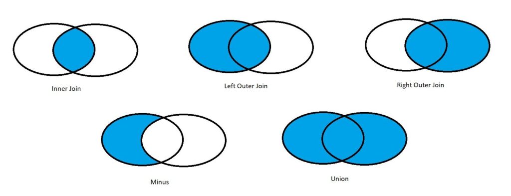
The diagram above shows Venn diagrams for different types of joins. This is of course not the exhaustive set, but for now we will live with this set.
- Inner Join/ Intersect
- This selects records that are common across two tables.
- Left Outer Join
- This will select everything from the left table even when records do not match in the right table.
- Right Outer Join
- Unlike left outer join, this picks up all records from right table even when records do not match on the left table.
- Minus
- This will select all distinct records from the left table and reject everything present in the right table.
- Union/ Full Outer Join
- This will combine all records from both tables and present
Let’s try some examples now to learn more about joins.
Q 1. Select top 10 employee number, first name, last name, gender and department name of employee sorted by employee number.
select e.emp_no, e.first_name, e.last_name, e.gender, t.title
  from employees.employees e
  join employees.titles t on t.emp_no = e.emp_no
 order by e.emp_no
 limit 10
;
| emp_no | first_name | last_name | gender | title |
|---|---|---|---|---|
| 10,001 | Georgi | Facello | M | Senior Engineer |
| 10,002 | Bezalel | Simmel | F | Staff |
| 10,003 | Parto | Bamford | M | Senior Engineer |
| 10,004 | Chirstian | Koblick | M | Engineer |
| 10,004 | Chirstian | Koblick | M | Senior Engineer |
| 10,005 | Kyoichi | Maliniak | M | Senior Staff |
| 10,005 | Kyoichi | Maliniak | M | Staff |
| 10,006 | Anneke | Preusig | F | Senior Engineer |
| 10,007 | Tzvetan | Zielinski | F | Senior Staff |
| 10,007 | Tzvetan | Zielinski | F | Staff |
This is an example of intersection or inner join. In this case we are joining two tables employees and titles on emp_no. Here you will also see an example of a table alias. Here we are aliasing employees as e and titles as t and using this aliases in query. It is very important to add table name alias to columns, because database parser may be confused what table to refer a column from.
There is a older way of writing this query also that you may see being used in a lot of places. Just to provide the context, I am also adding the second form of query.
select e.emp_no, e.first_name, e.last_name, e.gender, t.title
  from employees.employees e, employees.titles t
 where t.emp_no = e.emp_no
 order by e.emp_no
 limit 10
;
In this way of the query, we comma separate all tables and add all joins in where. For outer joins, that we learn in next sections, it uses different syntax for different databases. Most databases tend to use (+). But it is better to use the more descriptive newer format while writing queries.
Q 2. Find all employees sorted by employee number and find the department name where they work and identify their manager.
Now this question is a bit difficult. If you look at the table ER diagram, there is no direct relationship between employee and their managers. Employees are associated with a department and each department is assigned a manager. Every manager is again an employee. So, the query looks like this,
select e.emp_no, e.first_name, e.last_name, d.dept_name,
       e2.emp_no as mgr_no, e2.first_name as mgr_first_name, e2.last_name as mgr_last_name
  from employees.employees e
  join employees.dept_emp de on de.emp_no = e.emp_no and sysdate() between de.from_date and de.to_date
  join employees.departments d on d.dept_no = de.dept_no
  join employees.dept_manager dm on dm.dept_no = d.dept_no and sysdate() between dm.from_date and dm.to_date
  join employees.employees e2 on e2.emp_no = dm.emp_no
 order by e.emp_no
 limit 10
;| emp_no | first_name | last_name | dept_name | mgr_no | mgr_first_name | mgr_last_name |
|---|---|---|---|---|---|---|
| 10,001 | Georgi | Facello | Development | 110,567 | Leon | DasSarma |
| 10,002 | Bezalel | Simmel | Sales | 111,133 | Hauke | Zhang |
| 10,003 | Parto | Bamford | Production | 110,420 | Oscar | Ghazalie |
| 10,004 | Chirstian | Koblick | Production | 110,420 | Oscar | Ghazalie |
| 10,005 | Kyoichi | Maliniak | Human Resources | 110,228 | Karsten | Sigstam |
| 10,006 | Anneke | Preusig | Development | 110,567 | Leon | DasSarma |
| 10,007 | Tzvetan | Zielinski | Research | 111,534 | Hilary | Kambil |
| 10,009 | Sumant | Peac | Quality Management | 110,854 | Dung | Pesch |
| 10,010 | Duangkaew | Piveteau | Quality Management | 110,854 | Dung | Pesch |
| 10,012 | Patricio | Bridgland | Development | 110,567 | Leon | DasSarma |
In this case there are quite a lot of equijoins. We keep on adding a new table in each line and defining the relation till we have all tables that play a part in this query.
Before we proceed with the this query, we will add one more department to the departments table. This will be used to demonstrate outer join. If you are following through the tutorial, please make sure to add this to your database. We will add a new department known as Information Technology.
insert into employees.departments
values ('d010', 'Information Technology')
;
commit
;
Q 3. List departments without any employee.
This problem can be solved easily using a different solution, but because we want to demo outer join, we will solve it the outer join way. Let us see how outer join works. In case of outer joins, we will also bring in data from the table with additional data that has no match to the other table.
So, consider this query,
select d.dept_name, de.emp_no
  from employees.dept_emp de
  join employees.departments d on d.dept_no = de.dept_no
 where de.emp_no is null
;
If you see, we are trying to find any department that does not have an employee. However, since we did an inner join, we intersect the two tables and any record without employees did not even come in this query. So, resultset is empty.
However, if we can use a right outer join, and we indicate that right side of the query has additional data, we would be able to fetch it also. We know that we added Information Technology as department which does not have any employees.
select d.dept_name, de.emp_no
  from employees.dept_emp de
  right outer join employees.departments d on d.dept_no = de.dept_no
 where de.emp_no is null
;
| dept_name | emp_no |
|---|---|
| Information Technology |
So, doing a right outer join gives intended result. Left outer join behaves the same way. However, in that case we will say that left side of the join has excess data. We will not go too deep into these queries; you can try additional queries yourself.
Next, we will try to show a Union/ full outer join and finish this section. We will use UNION clause here but remember there is also something called UNION ALL. The difference is that UNION will return unique records, whereas UNION ALL will return duplicates.
Q 4. Find all employees born in either 1956 or 1965. Here we use a function called YEAR, we will learn about this later.
select * from (
select emp_no, birth_date, first_name, last_name
  from employees.employees e
 where year(birth_date) = 1956

union

select emp_no, birth_date, first_name, last_name
  from employees.employees e
 where year(birth_date) = 1965
) as a
order by 1
limit 10
;
| emp_no | birth_date | first_name | last_name |
|---|---|---|---|
| 10,014 | 1956-02-12 | Berni | Genin |
| 10,029 | 1956-12-13 | Otmar | Herbst |
| 10,033 | 1956-11-14 | Arif | Merlo |
| 10,042 | 1956-02-26 | Magy | Stamatiou |
| 10,055 | 1956-06-06 | Georgy | Dredge |
| 10,095 | 1965-01-03 | Hilari | Morton |
| 10,099 | 1956-05-25 | Valter | Sullins |
| 10,107 | 1956-06-13 | Dung | Baca |
| 10,122 | 1965-01-19 | Ohad | Esposito |
| 10,132 | 1956-12-15 | Ayakannu | Skrikant |
If you see the results above, we only got birthday years from 1956 and 1965. One thing to remember for Union is that the resulting columns returned by both queries should be the same count and have the same datatypes.
Remember that join is much broader than what has been defined above. You will have to play around different queries to learn them.
Aggregate functions – Group By
Group by clause is used for summarizing and printing values. We will start with an example.
Q 1. List count of employees by job title.
select t.title, count(t.emp_no)
  from employees.titles t
 group by t.title
 order by 2 desc
;
| title | count(t.emp_no) |
|---|---|
| Engineer | 115,003 |
| Staff | 107,391 |
| Senior Engineer | 97,750 |
| Senior Staff | 92,853 |
| Technique Leader | 15,159 |
| Assistant Engineer | 15,128 |
| Manager | 24 |
Let’s see what we are doing here. We are getting the count of employees for every job title, however, grouping it for each job title present. One think to note here is that every grouping has to be added to the group by clause below. Here we used count, but we could have used any aggregation functions we had defined earlier.
Let’s make it a little bit more complicated.
Q 2. List count of employees by job title under each department.
select d.dept_name, t.title, count(de.emp_no)
  from employees.titles t
  join employees.dept_emp de on de.emp_no = t.emp_no and sysdate() between de.from_date and de.to_date
  join employees.departments d on d.dept_no = de.dept_no
 where sysdate() between t.from_date and t.to_date
 group by d.dept_name, t.title
 order by 1, 2
;
| dept_name | title | count(de.emp_no) |
|---|---|---|
| Customer Service | Assistant Engineer | 68 |
| Customer Service | Engineer | 627 |
| Customer Service | Manager | 1 |
| Customer Service | Senior Engineer | 1,790 |
| Customer Service | Senior Staff | 11,268 |
| Customer Service | Staff | 3,574 |
| Customer Service | Technique Leader | 241 |
| Development | Assistant Engineer | 1,652 |
| Development | Engineer | 14,040 |
| Development | Manager | 1 |
| Development | Senior Engineer | 38,816 |
| Development | Senior Staff | 1,085 |
| Development | Staff | 315 |
| Development | Technique Leader | 5,477 |
| Finance | Manager | 1 |
| Finance | Senior Staff | 9,545 |
| Finance | Staff | 2,891 |
| Human Resources | Manager | 1 |
| Human Resources | Senior Staff | 9,824 |
| Human Resources | Staff | 3,073 |
| Marketing | Manager | 1 |
| Marketing | Senior Staff | 11,290 |
| Marketing | Staff | 3,551 |
| Production | Assistant Engineer | 1,402 |
| Production | Engineer | 12,081 |
| Production | Manager | 1 |
| Production | Senior Engineer | 33,625 |
| Production | Senior Staff | 1,123 |
| Production | Staff | 349 |
| Production | Technique Leader | 4,723 |
| Quality Management | Assistant Engineer | 389 |
| Quality Management | Engineer | 3,405 |
| Quality Management | Manager | 1 |
| Quality Management | Senior Engineer | 9,458 |
| Quality Management | Technique Leader | 1,293 |
| Research | Assistant Engineer | 77 |
| Research | Engineer | 830 |
| Research | Manager | 1 |
| Research | Senior Engineer | 2,250 |
| Research | Senior Staff | 9,092 |
| Research | Staff | 2,870 |
| Research | Technique Leader | 321 |
| Sales | Manager | 1 |
| Sales | Senior Staff | 28,797 |
| Sales | Staff | 8,903 |
Let’s take one more example.
Q 3. Get the average salary for each gender.
select e.gender, truncate(avg(s.salary), 2)
  from employees.salaries s
  join employees.employees e on e.emp_no = s.emp_no
 where sysdate() between s.from_date and s.to_date
 group by e.gender
;
| gender | truncate(avg(s.salary), 2) |
|---|---|
| M | 72,044.65 |
| F | 71,963.57 |
One additional thing of interest here. We have used a MySQL function TRUNCATE here. This was used to restrict the values for the salary average to 2 decimal places. There are a lot of other such functions that MySQL provide. At the time of writing, you can access all of these function list here.
MySQL :: MySQL 8.0 Reference Manual :: 12.1 Built-In Function and Operator Reference
Let’s restrict this is to a specific departments.
Q 4. Get the average salary for each gender for departments d001 and d002.
select de.dept_no, e.gender, truncate(avg(s.salary), 2)
  from employees.salaries s
  join employees.employees e on e.emp_no = s.emp_no
  join employees.dept_emp de on de.emp_no = e.emp_no and sysdate() between de.from_date and de.to_date
 where sysdate() between s.from_date and s.to_date
 group by de.dept_no, e.gender
 having de.dept_no in ('d001', 'd002')
;| dept_no | gender | truncate(avg(s.salary), 2) |
|---|---|---|
| d001 | F | 79,699.77 |
| d001 | M | 80,293.38 |
| d002 | F | 78,747.41 |
| d002 | M | 78,433.3 |
We have introduced a new clause here, HAVING. The difference between HAVING and WHERE is that HAVING filters within the group and is hence more efficient.
CASE statements
We will take CASE as a separate heading, as it is sometimes required for evaluation and printing data based on some queries.
Q 1. List all employees with their salaries. Additionally, state the following,
- If salary is less than 60K, label as Grade 1
- If salary is greater than 60K but less than 120K, label as Grade 2
- All others label as Grade 3
select concat(e.last_name, ', ', e.first_name) as "Name", s.salary as "Salary",
  case
  	when s.salary < 60000 then 'Grade 1'
  	when s.salary between 60000 and '120000' then 'Grade 2'
  	else 'Grade 3'
  end as "Grade"
  from employees.salaries s
  join employees.employees e on e.emp_no = s.emp_no
 where sysdate() between s.from_date and s.to_date
  limit 15
;
| Name | Salary | Grade |
|---|---|---|
| Facello, Georgi | 88,958 | Grade 2 |
| Simmel, Bezalel | 72,527 | Grade 2 |
| Bamford, Parto | 43,311 | Grade 1 |
| Koblick, Chirstian | 74,057 | Grade 2 |
| Maliniak, Kyoichi | 94,692 | Grade 2 |
| Preusig, Anneke | 59,755 | Grade 1 |
| Zielinski, Tzvetan | 88,070 | Grade 2 |
| Peac, Sumant | 94,409 | Grade 2 |
| Piveteau, Duangkaew | 80,324 | Grade 2 |
| Bridgland, Patricio | 54,423 | Grade 1 |
| Terkki, Eberhardt | 68,901 | Grade 2 |
| Genin, Berni | 60,598 | Grade 2 |
| Cappelletti, Kazuhito | 77,935 | Grade 2 |
| Bouloucos, Cristinel | 99,651 | Grade 2 |
| Peha, Kazuhide | 84,672 | Grade 2 |
Conclusion
That was a long one. Hope you find this useful as a reference. Ciao for now!