In the inaugural post of this series, we explored the fascinating transition from Traditional AI to Agentic AI. As we continue this journey, let’s take a moment to delve into the realm of Language Models. We will examine how it started from statistical models and then a pivotal paper published by Google in 2017 revolutionized the way we generate “next tokens” in AI language processing.
This exploration not only enhances our understanding of Language Models but also sets the stage for the advanced capabilities we see in Agentic AI today. So onward and upward we go.
What is a Language Model?
A language model in terms of Artificial Intelligence is a model that can understand and generate human language. Trained on a huge corpus (collection) of data, these models can predict the next “token” that is most likely based on one or more words provided. These models are used for text generation, language translation or speech recognition tasks.
Tokens
We have been talking about tokens for sometime now. What is a token? Tokens are parts of the word broken down by semantic meaning. Each of these chunks can be of variable length and as such a punctuation mark will hold on its own as a distinct token. Let’s take an example.
Learning about agent in AI is fun.
So, what are the tokens in this? Again, it’s not that simple. There are different types of tokens that can be used.
- Word Tokens: This is the most simplistic. Every word in this case is a token. So, for our example, it will be split as: Learning / about / agent / in / AI / is / fun / .
- Subword Tokens: Most language models in use today will tokenize based on semantic meaning. In this case words may be broken down in smaller pieces. So, we will get: Learn / ing / about / agent / in / AI / is / fun / .
- Character Tokens: In some cases, we will have individual characters as tokens.
- Punctuation Tokens: If there are punctuations in the sentences, they will be split in its own token.
- Special Tokens: This indicates start of text marker, end of text marker, unknown text marker to name a few.
In OpenAI GPT models, that sentence above will have 8 tokens.
Learning | ␣about | ␣agent | ␣in | ␣AI | ␣is | ␣fun | .
Now let’s learn about one of the older language models.
N-gram language model
Imagine you are on your phone typing in words. You see that next recommended words keep on getting displayed at the bottom of the screen. How does this work? To understand, let’s discuss about one of the primitive model.
N-grams refer to a sequence of words that is used to build a language model. Here N refers to the number of words in the sequence. So, if we have a 2 word sequence, we call it a bigram, a 3 word sequence is called a trigram and so on. Taking the example on top,
Learning about agent in AI is fun.
Following are the bigrams we can extract.
Learning about
about agent
agent in
in AI
AI is
is fun.
Following are the trigrams that can be extracted.
Learning about agent
about agent in
agent in AI
in AI is
AI is fun.
Markov Chains
Bigrams, trigrams kind of models can be used with one of the statistical models known a Markov Chains to predict next word in sequence.
Let’s take the following four sentences and draw a Markov chain for that. We will assume that all of these have equal probabilities of happening.
1. Today is cloudy
2. Today is humid and sultry
3. Today is humid and cold
4. Today is cloudy and humid
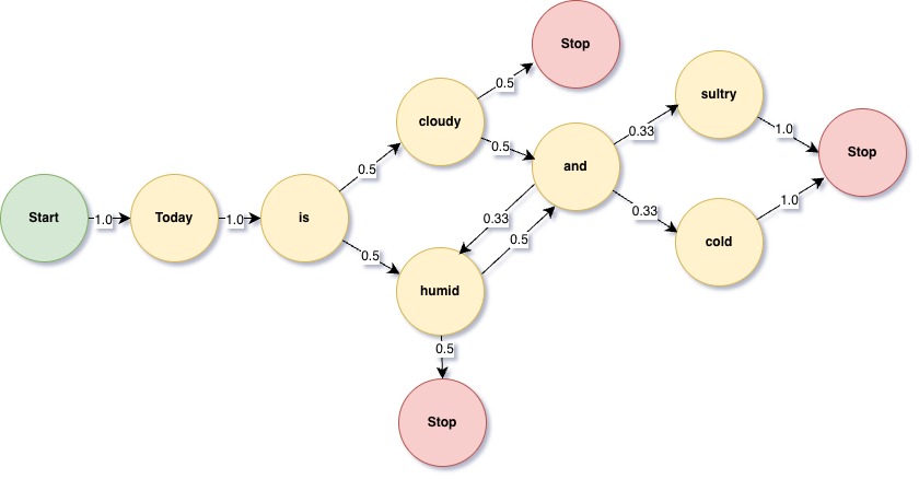
Above diagram shows the Markov Chain for the four sentences. The way it works is that we will find all next words for a specific word and distribute based on how paths are there to next words.
For a bigram, we know the next word will depend on the last word and any of the path can be traversed. So, all of these are valid sentences.
1. Today is humid.
2. Today is cloudy.
3. Today is cloudy and sultry.
4. Today is cloudy and cold.
5. Today is cloudy and humid.
6. Today is humid and cold.
7. Today is humid and sultry.
8. Today is humid and humid ????
So, for bigrams, the next word only depends on previous word (or per Markov’s rules, previous state).
def generate_ngrams(self, n, txt):
        """
        This method can be used to generate n-grams

        :param n: N gram
        :param txt: Text to get N-gram
        """
        words = txt.split()

        if len(words) < n:
            return {}

        # Generate n-grams
        ngrams = [tuple(words[i:i+n]) for i in range(len(words)-n+1)]

        # Count occurrences of each (n-1)-gram and their following word
        context_counts = defaultdict(Counter)
        for ngram in ngrams:
            context, next_word = tuple(ngram[:-1]), ngram[-1]
            context_counts[context][next_word] += 1

        # Calculate probabilities
        probabilities = {}
        for context, next_words_count in context_counts.items():
            total_occurrences = sum(next_words_count.values())
            probabilities[context] = {word: count / total_occurrences for word, count in next_words_count.items()}

        return probabilities
This method can generate bigrams given a sentence. Since we are interested in bigrams only, we can send 2 as n and for this example I sent Moby Dick text downloaded from Project Gutenberg. To predict a next word, we can do the following,
def predict_next_word(self, bigram, vals):
        """
        Predict the next string based on the last two. At this point we are considering bigrams

        :param bigram: Bigram tuple
        :param vals: All the bigrams
        """
        nextwords = vals.get(bigram)
        if not nextwords:
            return None

        words, probs = zip(*nextwords.items())
        word = random.choices(words, weights=probs)[0]
        return word
So, if I generate 50 word sentence starting with “the boat”, here is a sample.
the boat steerer or harpooneer is stark mad and steelkiltbut gentlemen you shall hear it was plainly descried from the beginning all this seemed natural enough especially as they do hills about boston to fill the scuttlebutt near the door i dont fancy having a man might rather have done
Pretty random I would say. But then came deep learning to the rescue.
Recurrent Neural Network (RNN)
RNN as the name suggests is a neural network that addressed some of the problems that Markov chains had. It can capture sequential data within a limit and can be used for NLP tasks. It is also context aware as it can maintain state information.
RNN maintains hidden layers (recurrent unit) that keeps information about the previous inputs and for each step also uses a feedback loop to learn from previous states. However there is a limit to how much information it can store and at some point memory starts to fade. This is called the vanishing gradient problem. Also RNN always has to process data in sequence and the next state will contain information about previous states. This is the reason we cannot do any parallel processing during training of these neural networks.
This problem of vanishing gradients is solved by a model called LSTM (Long Short Term memory) that adds the ability to also forget anything that is learned and not needed. This way it can store more information about previous states.
GRU (Gated Recurrent Units) were introduced later that were more computationally efficient than their counterparts LSTM. It is not in the scope of this blog to go into further details about all of these architectures as each one will need a dedicated blog by itself, so we will leave it at this 10,000 feet view.
Sample RNN
To demonstrate we will create a simple RNN using PyTorch (reusing the RNN model that PyTorch provides). All codes will be in GitHub (https://github.com/chakrab/suvcodes). The model looks like below.
 import torch.nn as nn

class RNNModel(nn.Module):
    """
    A simple Recurrent Neural Network (RNN) model for sequence prediction tasks.
    It consists of an embedding layer, an RNN cell, and a fully connected layer.
    Attributes:
        vocab_size (int): The size of the vocabulary.
        embedding_dim (int): The dimensionality of the embedded words.
        hidden_dim (int): The number of units in the hidden state.
    Methods:
        forward(x): The forward pass through the network. It takes an input tensor x and returns a predicted output tensor.
    """
    def __init__(self, vocab_size, embedding_dim, hidden_dim):
        super(RNNModel, self).__init__()
        self.embedding = nn.Embedding(vocab_size, embedding_dim)
        self.rnn = nn.RNN(embedding_dim, hidden_dim, batch_first=True)
        self.fc = nn.Linear(hidden_dim, vocab_size)

    def forward(self, x):
        x = self.embedding(x)
        out, _ = self.rnn(x)
        out = self.fc(out)
        return out
To load data to this model, we will need to create a corpus. We can read the same ebook, sanitize text, tokenize using NLTK library and finally wrap it in a python dataset. So key parts of my data loader will look as below.
def load_data(self):
        """
        Loads data from the specified file path.

        This method reads the text from the file, tokenizes it into words,
        and stores the result in the `corpus` attribute of the class instance.

        Note: The downloaded 'punkt' package is required for word tokenization.
        """
        with open(self.file_path, 'r') as file:
            text = file.read()[:10000]
            nltk.download('punkt')
            self.corpus = word_tokenize(text.lower())

def build_vocab(self):
        """
        Builds the vocabulary of the corpus by counting the occurrences of each word.

        Returns:
            None
        """
        counter = Counter(self.corpus)
        self.word_to_idx = {word: idx for idx, (word, _) in enumerate(counter.items())}
        self.idx_to_word = {idx: word for word, idx in self.word_to_idx.items()}
Primary training block is given below/
def train(self, device):
        """
        Trains the RNN model on the training dataset.

        Args:
            device (torch.device): The device to use for training (e.g., Metal or CPU).

        Returns:
            None
        """
        for epoch in range(self.epochs):
            start = time.time()
            for inputs, targets in self.train_loader:
                inputs, targets = inputs.to(device), targets.to(device)
                self.optimizer.zero_grad()
                outputs = self.model(inputs)
                loss = self.criterion(outputs.view(-1, outputs.size(2)), targets.view(-1))
                loss.backward()
                self.optimizer.step()
            end = time.time()
            print(f'Epoch {epoch + 1}/{self.epochs}, Loss: {loss.item()}, time (s): {end - start}')
Eventually after running for quite some time, depending on your GPU speed and corpus size, we will get a model that can be retrieved at a later state. I ran this training on first 10,000 words and asked to generate a sentence. Remember a 10,000 words corpus is fairly small. I asked to generate 5 words after “love of”. This is what was generated: love of oil swimming in the ocean. Well that does not make too much of a sense either, but this simple model was only trained on a limited subset.
RNN and LSTM were game changers in the field till in 2017 when one of the landmark papers was introduced by eight scientists working at Google.
Attention is All you Need
In June of 2017, a landmark paper titled “Attention is All You Need” was proposed by Vaswani et al. changing how we think about Natural Language Processing (NLP) and bringing a new architecture termed as “Transformers”. They demonstrated how the Attention mechanisms can replace Recurrent layers to efficiently handle deductions of sequences without relying on sequential computations.
The core innovation of this paper is the self-attention mechanism, which enables the model to weigh the influence of different words in a sentence dynamically, allowing it to focus on relevant parts of the input data regardless of their position. This allows the model to analyze long-range dependencies better than RNN or LSTM. Think about the sentences below:
1. This bank will be closed tomorrow.
2. I will talk to the banker tomorrow to understand stock market.
3. The wedding would be held on the banks of river Thames.
4. I always bank on my own judgement instead of unrealistic theories.
In the sentences above each of the bank puts a different meaning to the word. It all depends on the context where it is used. The transformer model uses “scaled dot product” attention layers combined with multi-head attention to capture each of these different meanings in their appropriate context. Additionally it adds positional encodings to also store the order of tokens. In this case, all recurrent layers are removed and replaced with attention layers.
Transformers
This is the proposed architecture as defined in the research paper that was published from Google. We will not go over all the details here because the intent is to provide high level path to Transformer models.
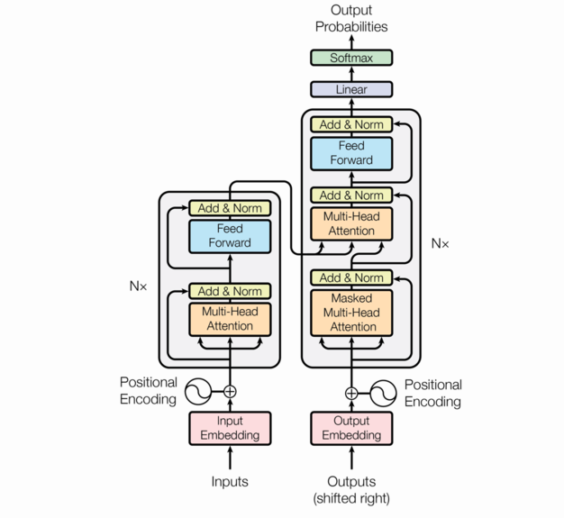
As we said earlier, Transformers use attention mechanism to predict the next word. Eventually what we get is a probability list of next words following the sentence that is already formed within the models context window. We can change the randomness of this selection by providing a bigger value of what is called temperature. And then what happens is sheer magic and lo and behold a meaningful sentence is generated.
The efficiency and scalability of these transformers paved the way to modern AI models. Currently transformer models are used for translations (original intent), chat generation, image to text, text to image, audio generation and a lot more.
We will not go into full details, but there are some key concepts that are worth documenting in relation to transformers.
Embeddings
While not necessarily a transformer concept, but all input has to be converted to numeric values based on tokens. Each token generates a separate number. So, bank and Bank will be two different encodings. When an input is received, it is converted to a vector of numbers. This is what is required to train the model. Eventually, when a response is generated, it also gets generated as a sequence of embeddings and converted back to corresponding word and displayed.
Self Attention
Self Attention is primarily three sets of vectors calculated during training to and part of attention. Each embedding is multiplied with these three vector and a final score is calculated.
- Query (Q) vector: This vector calculates the relevance of this word with other word. This is more like What is asked?
- Key (K) vector: This is the meaning or the object of query in question. It is not really What, but it identifies the context what needs to be mapped.
- Value (V) vector: After the point of attention is received, value will represent the actual information this token carries. This is weighed in with the Q and V vector.
Eventually we get an attention score after multiplying with calculated/ adjusted weights.
Multi-Head Attention
Transformers do not just limit to a single Self Attention. It will calculate multiple attentions at the same time. Each of these heads will capture a different relationship.
Positional Understanding
Unlike RNN, attention data does not keep the positional information. This is also added as a layer to maintain what positions a word can exist in with respect to other words.
Softmax Layer
This layer makes sure that all probabilities are normalized and eventually add up to 1. It’s a standard algorithm used across a lot of machine learning models.
Encoder/ Decoder
This is one of the key process in Transformer mechanism. Encoder will take a sentence and create the equivalent vector representation. Decoder does just the opposite. It can take a vector and creates the corresponding sentence. Each encoder/ decoder will include an attention layer and feed-forward layers.
That’s more or less the key concepts for Transformer.
Conclusion
The evolution from Markov chains to Transformers illustrates the rapid advancements in language modeling techniques. Each stage of development has built upon the previous ones, addressing limitations and introducing new capabilities. As we stand on the brink of further innovations, it’s clear that the journey of LLMs is far from over. The future promises even more sophisticated models capable of deeper understanding and broader applications in natural language processing. However, it’s far from over. As researchers keep on exploring new frontiers, Artificial Intelligence will keep on moving forward. Ciao for now!
1 thought on “Language Models: Markov Chains to Transformers”
Comments are closed.