One of the major problems in logistics is the optimal path problem. Imagine you are a delivery driver and have been tasked to deliver packages in twenty-five different places in New York City. How do you calculate the optimum route that you should drive so that your time taken is minimum? Ignoring external factors like traffic jams, and considering the road speeds, you will try to optimize so that most of travel covers wider avenues than local streets. But that is just one part of the problem.
This problem is really two problems disguised in one.
- Pathfinding. How far is it from stop A to stop B? That is a shortest-path question on the road network.
- Ordering. Given the distance between every pair of stops, in which order should I visit them? That is the travelling salesman problem (TSP).
Today in this blog, we will go through the first part of the problem aka. Pathfinding problem. We will go over four algorithms most widely used across the industry. Before we delve deep into it, let’s see how the algorithms affect optimal time.
The Algorithms
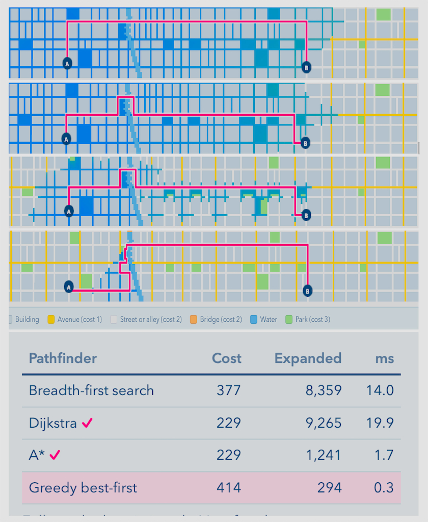
In this image, we are graphing the four algorithms we will discuss. Imagine a city with avenues, streets and areas with more crowds. A river flows through it only allowing traffic over some bridges. We have points associated with each of them based on speed and traffic.
Each algorithm tried a different approach to arrive at a route. Only two of them are optimal. So, how are these calculating the routes?
The first graph is Breadth First Search (BFS). In this case it ignores the costs (or weights) assigned to each road, and tries to always calculate the shortest route (least number of edges). So, in this case, it spent a lot of time on the streets, taking it’s score up – thus was not optimal cost (but achieved least hops).
The second graph is Dijkstra. This considered the weights of the roads and optimized the route based on total score. Even though it traversed a lot of the graph, it still came up with the most optimal routing.
The third is A*. This keeps all the benefits of the above, but uses heuristics to traverse less path. The only issue with this algorithm is that if we do not have a proper heuristic function, the route will not be optimal.
The fourth one is greedy and uses heuristics to force towards the destination. It may not always be optimal. As you can see in the diagram, it went straight towards the destination, hit the river and had to step back towards the bridge. This increased the score quite a bit.
The image also contains a benchmark comparison between the four algorithms. Take a look at the metrics (Cost: Sum of all Weights, Expanded: How many cells were opened, ms: milliseconds).
The Problem
We will make one more stop before going to the details. Let’s first define our own city with some houses. Each house leads to one or more other houses. Based on where you are coming from you have to pay toll when you go to the house. Our target will be to go to the destination with the minimum toll paid. The coordinates are needed to calculate the distance between the houses.
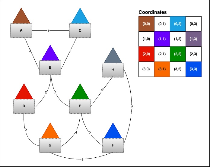
There are multiple problems finding a path here as the costs are not optimized. To go from A -> G, the cheapest path is not the shortest. Direct traversal to B and following the path is more expensive than taking a long way through C. Same happens from B to G. The longest route is the smallest cost. The ideal path is:
A -> C -> B -> E -> F -> G (cost: 7)
We will build our algorithms based on the image above.
Breadth First Search (BFS)
BFS explores a graph one layer at a time: first the start node’s neighbors, then nodes two edges away, and so on. It finds a path with the fewest edges in an unweighted graph – or when every edge has the same cost.
BFS does not respect any cost, however it will calculate the least number of steps. So if I want to move from house A to house G, BFS will find the shortest path. It is used when you do not bother about weights, or all weights are the same. For our house example above, let’s write the step-by-step frontier expansion using BFS.
What does step-by-step frontier expansion table depict? The frontier is the set of discovered-but-unexplored nodes, typically held in a queue or priority queue. Expanding a node means pulling it from the frontier and examining its neighbors, adding any new ones to the frontier. The order of expansion is what defines each algorithm — BFS explores oldest-first, Dijkstra expands the cheapest node, A* expands the most promising, and greedy rushes toward the goal. In short, expansion is the engine that drives the search forward toward the goal.
| Step | Expanded | Frontier | Visited |
|---|---|---|---|
| 1 | A | B, C | A, B, C |
| 2 | B | C, D, E | A, B, C, D, E |
| 3 | C | D, E | A, B, C, D, E |
| 4 | D | E, G | A, B, C, D, E, G |
| 5 | E | G, F, H | A, B, C, D, E, F, G, H |
| 6 | G | F, H | A, B, C, D, E, F, G, H |
BFS path: ['A', 'B', 'D', 'G'] cost: 10, hops: 3 (optimized)
Use Cases
Some sample use cases for this algorithm,
- Finding the closeness of two people in a social network (get hop count).
- Find minimum number of moves between two points in a simple puzzle.
- Discovering every point in a puzzle that is lower than a certain number of steps.
- Explore any unweighted graphs.
We should not use BFS when edges have different costs, for example when roads have tolls, differ in distance or speed etc.
Dijkstra
Dijkstra’s algorithm tracks the total cost of reaching each node and explores the least-cost option next. It finds shortest paths when edge costs are non-negative. It’s a strong choice when costs vary and you don’t have a useful estimate of the distance to the destination.
Dijkstra’s algorithm repeatedly selects the unvisited node with the smallest known cost, then relaxes its outgoing edges: it updates a neighbor’s distance if going through that node gives a cheaper path.
Let’s check the logical step-by-step frontier expansion,
| Step | Expanded | g | Frontier node(g) | Expanded order |
|---|---|---|---|---|
| 1 | A | 0 | C(1), B(3) | A |
| 2 | C | 1 | B(2) | A, C |
| 3 | B | 2 | D(4), E(4) | A, C, B |
| 4 | D | 4 | E(4), G(9) | A, C, B, D |
| 5 | E | 4 | F(6), G(8), H(8) | A, C, B, D, E |
| 6 | F | 6 | G(7), H(8) | A, C, B, D, E, F |
| 7 | G | 7 | H(8) | A, C, B, D, E, F, G |
Dijkstra path: ['A', 'C', 'B', 'E', 'F', 'G'] cost: 7
We used a term called Relax. In graph theory, the Edge Relaxation property is defined as updating a path to the least cost when there are multiple paths to the same node. For example, in our example above, for A -> B, it is better to traverse A -> C -> B. In this case, the path will be updated to later.
Use Cases
- Finding the lowest cost path through a weighted network.
- Calculating the shortest path from one starting point to many destinations.
- Routing when links have different costs, like latency or distance.
This algorithm cannot be used when an edge has negative cost. This does iterate a lot of area around the path, so it may feel slower. Most cases will work better with A*.
A* search
A* combines current cost and using heuristics estimates remaining cost. It uses both the route so far and a prediction of what remains. With non-negative edge costs and an appropriate heuristic, A* can find an optimal path; however it relies on the heuristic to not overestimate cost. Normally we use Euclidean distance or Manhattan distance to calculate the remaining path. We will use Manhattan distance because it is easier to calculate manually if you want to wrap your head around the expansion table. For cities, most of the time Manhattan distance is the one that is preferred as they have a grid-like layout of avenues and streets.
Euclidean distance represents the shortest straight-line distance between two points in Euclidean space. It is the easiest to understand and most used metric to calculate distance. Distance is calculated as follows:

d = √((x2 - x1)2 + (y2 - y1)2)

Manhattan distance, also called Taxicab or City Block distance, calculates the sum of the absolute differences of Cartesian coordinates.

d = |x2 - x1| + |y2 - y1|

We normally use Manhattan distance for A* algorithms because it is better suited for grid-like paths that are restricted to mostly horizontal and vertical paths. Since our example has quite a few diagonals, Euclidean distance is a better fit. Manhattan distance is admissible, but on graphs with shortcut edges (where an edge weight is smaller than the implied distance), it is inconsistent. Closed-set A* with an inconsistent heuristic can return a suboptimal path — here it returns cost 8 instead of 7. Using re-expansion restores the optimality guarantee.

To be guaranteed optimal, heuristic for A* should be:

  1. Admissible - never overestimates
  2. Consistent — satisfies the triangle inequality along edges

For our graph, Manhattan is admissible but NOT consistent.
Here is the frontier expansion table when we used the Manhattan distance,
| Step | Expanded | g | h | f | Frontier node(f) | Closed order |
|---|---|---|---|---|---|---|
| 1 | A | 0 | 4 | 4 | B(5), C(5) | A |
| 2 | B | 3 | 2 | 5 | C(5), D(7), E(7) | A, B |
| 3 | C | 1 | 4 | 5 | D(7), E(7) | A, B, C |
| 4 | D | 5 | 2 | 7 | E(7), G(10) | A, B, C, D |
| 5 | E | 5 | 2 | 7 | F(9), G(9), H(13) | A, B, C, D, E |
| 6 | F | 7 | 2 | 9 | G(8), H(13) | A, B, C, D, E, F |
| 7 | G | 8 | 0 | 8 | H(13) | A, B, C, D, E, F, G |
A* path (closed, Manhattan): ['A', 'B', 'E', 'F', 'G'] cost: 8
Re-expansion A*
The problem with A* is that it is normally closed order and only returns the optimal path when the heuristic is proper. We can modify the algorithm to look back nodes and reopen if a better path is found. There is no universally accepted name for this, but one common name is called A* with re-expansion. This maintains the g value and can reopen nodes when cost decreases. If we create this, the frontier expansion changes,
| Step | Expanded | g | h | f | Frontier node(f) | Expanded order |
|---|---|---|---|---|---|---|
| 1 | A | 0 | 4 | 4 | B(5), C(5) | A |
| 2 | C | 1 | 4 | 5 | B(4) | A, C |
| 3 | B | 2 | 2 | 4 | D(6), E(6) | A, C, B |
| 4 | D | 4 | 2 | 6 | E(6), G(9) | A, C, B, D |
| 5 | E | 4 | 2 | 6 | F(8), G(8), H(12) | A, C, B, D, E |
| 6 | F | 6 | 2 | 8 | G(7), H(12) | A, C, B, D, E, F |
| 7 | G | 7 | 0 | 7 | H(12) | A, C, B, D, E, F, G |
A* path (optimized, Manhattan): ['A', 'C', 'B', 'E', 'F', 'G'] cost: 7
Use Cases
- Finding a route to a specific destination on a map.
- Pathfinding in games or robotics when movement costs vary.
- Search problems where a useful heuristic can guide exploration without sacrificing the desired optimalityguarantee.
A* should not be used if a suitable heuristic is not available. It will not provide optimal results.
Greedy Best-First Search
Greedy Best-First Search chooses the node that appears closest to the goal according to a heuristic. Unlike A* it ignores the cost that has already been paid to reach the node. This makes it very fast, but the route may not be optimal.
We give below the frontier expansion table,
| Step | Expanded | h | Frontier node(h) | Expanded order |
|---|---|---|---|---|
| 1 | A | 4 | B(2), C(4) | A |
| 2 | B | 2 | D(2), E(2), C(4) | A, B |
| 3 | D | 2 | G(0), E(2), C(4) | A, B, D |
| 4 | G | 0 | E(2), C(4) | A, B, D, G |
Greedy path: ['A', 'B', 'D', 'G'] cost: 10
Use Cases
- Finding a possible route quickly when an exact optimum is not essential.
- Search tasks where a useful heuristic points strongly toward the goal.
- Applications where a fast, “good enough” answer is more valuable than proving it is best.
Quick Decision Guide
- Edges have no cost/ costs the same: BFS
- Costs vary, and do not have a proper heuristic that can be used: Dijkstra
- Speed matters more than the cheapest route: Greedy Best-First
- Cheapest path to a goal, and you have a heuristic function: A*
Time/ Space Complexity
| Algorithm | Time Complexity | Space Complexity |
|---|---|---|
| Breadth-First Search | O(V + E) | O(V) |
| Dijkstra’s Algorithm | O(V + E) log V) | O(V) |
| A* Search | O (worst: O(bd) | O(V) |
| Greedy Best-First Search | O(V + E) | O(V) |
- V: Number of Vertices
- E: Number of Edges
- b: Branching factor
- d: Depth of the shallowest goal
Implementations
Any tech blog is incomplete without implementations. Even though I normally start with implementations, in this case, I deferred it to last. With the advent of fine AI models, manual coding has taken a step back. We can still build beautiful programs without understanding anything remotely about coding.
But here it is, Python-based code implementations for these. And I will show you couple of methods for A* and describe each one.
Let’s define two structures to keep the path and coordinates.
def __init__(self):
  """Set up the sample graph (path_graph) and the node coordinates
  used by the heuristic."""
  # Adjacency list: node -> list of (neighbor, edge weight)
  self.path_graph = {
    "A": [("B", 3), ("C", 1)],
    "B": [("D", 2), ("E", 2)],
    "C": [("B", 1)],
    "D": [("G", 5)],
    "E": [("F", 2), ("G", 4), ("H", 4)],
    "F": [("G", 1), ("H", 5)],
    "G": [],
    "H": []
  }

  # Node -> (x, y) position, used by A* and greedy to estimate
  # distance to the goal
  self.coords = {
    "A": (0,0),
    "B": (1,1),
    "C": (0,2),
    "D": (2,0),
    "E": (2,2),
    "F": (3,3),
    "G": (3,1),
    "H": (1,3)
  }
BFS
def bfs_path(self, start, goal, debug=False):
        """
        Breadth-first search over self.path_graph, ignoring edge weights.

        Finds the path with the fewest edges (not necessarily the lowest weight).

        Args:
            start: node to begin at.
            goal: node to reach.
            debug: if True, print a step-by-step table of the queue after each expansion.

        Returns:
            (path, cost): path is the list of nodes from start to goal and cost is the
            number of edges in it. Returns (None, inf) if goal is unreachable.
        """
        queue = deque([start])
        visited = {start}
        parent = {start: None}
        rows = []  # debug table rows

        while queue:
            node = queue.popleft()
            if node == goal:
                if debug:
                    rows.append([len(rows) + 1, node, self._fmt_frontier(queue), ", ".join(sorted(visited))])
                break

            for nbr, _ in self.path_graph.get(node, []):
                if nbr not in visited:
                    visited.add(nbr)
                    parent[nbr] = node
                    queue.append(nbr)

            if debug:
                rows.append([len(rows) + 1, node, self._fmt_frontier(queue), ", ".join(sorted(visited))])

        if debug:
            self._print_table(f"BFS {start} -> {goal}", ["Step", "Expanded", "Frontier (queue)", "Visited"], rows)

        if goal not in parent:
            return None, float("inf")

        # Reconstruct path
        path = []
        cur = goal
        while cur is not None:
            path.append(cur)
            cur = parent[cur]
        path.reverse()

        cost = len(path) - 1  # number of edges
return path, cost- Uses a queue (FIFO) to process nodes in order of discovery.
- Marks each node as visited the first time it’s seen — never revisited.
- Records a “parent” for every new node so the path can be traced back.
- Once the goal is found, walk backward through parent pointers.
- Reverse the result to produce the final start → goal path.
Dijkstra
def dijkstra_path(self, start, goal, debug=False):
        """
        Dijkstra's shortest-path search over self.path_graph.

        Always expands the unvisited node with the lowest known distance from start,
        so it finds the minimum total weight path (weights must be non-negative).

        Args:
            start: node to begin at.
            goal: node to reach.
            debug: if True, print a step-by-step table of the frontier after each expansion.

        Returns:
            (path, cost): path is the list of nodes from start to goal and cost is the
            minimum total edge weight. Returns (None, inf) if goal is unreachable.
        """
        pq = [(0, start)]
        dist = {start: 0}
        parent = {start: None}
        visited = set()
        order = []  # expansion order, for the debug table
        rows = []   # debug table rows

        while pq:
            cur_dist, u = heapq.heappop(pq)
            if u in visited:
                continue
            visited.add(u)
            order.append(u)

            if u == goal:
                if debug:
                    frontier = sorted(((v, d) for d, v in pq if v not in visited and d == dist[v]), key=lambda e: (e[1], e[0]))
                    rows.append([len(rows) + 1, u, cur_dist, self._fmt_frontier(frontier), ", ".join(order)])
                break

            for v, w in self.path_graph.get(u, []):
                if v in visited:
                    continue
                new_dist = cur_dist + w
                if new_dist < dist.get(v, float("inf")):
                    dist[v] = new_dist
                    parent[v] = u
                    heapq.heappush(pq, (new_dist, v))

            if debug:
                # Only live entries: not yet expanded and matching the best known distance
                frontier = sorted(((v, d) for d, v in pq if v not in visited and d == dist[v]), key=lambda e: (e[1], e[0]))
                rows.append([len(rows) + 1, u, cur_dist, self._fmt_frontier(frontier), ", ".join(order)])

        if debug:
            self._print_table(f"Dijkstra {start} -> {goal}",
                              ["Step", "Expanded", "g", "Frontier node(g)", "Expanded order"], rows)

        if goal not in parent:
            return None, float("inf")

        # Reconstruct path
        path = []
        cur = goal
        while cur is not None:
            path.append(cur)
            cur = parent[cur]
        path.reverse()

return path, dist[goal]- Greedily expands the unvisited node with the lowest known distance from the start.
- This “cheapest-so-far first” strategy guarantees the shortest total cost.
- Uses a priority queue (min-heap) to always pick the nearest unexplored node.
- For each neighbor, checks if a cheaper route was found — if so, updates distance and re-prioritizes.
- When goal isfound, walk backward from the goal through parent pointers to reconstruct the path.
- Return the path and its total cost (
dist[goal]).
A* (closed)
def astar_closed_path(self, start, goal, use_manhattan, debug=False):
        """
        A* search over self.path_graph using self.coords for the heuristic, with a closed set.

        Expands the node with the lowest f(n) = g(n) + h(n), where g is the cost so far
        and h is the Manhattan or Euclidean distance to goal. Once a node is expanded it is
        closed and never revisited, so the path is only guaranteed to be minimum-weight if
        the heuristic is consistent. With an inconsistent heuristic (e.g. Manhattan on this
        graph) it can return a costlier path; see astar_path for the version that fixes this.

        Args:
            start: node to begin at.
            goal: node to reach.
            use_manhattan: if True use the Manhattan heuristic, otherwise Euclidean.
            debug: if True, print a step-by-step table of the frontier after each expansion.

        Returns:
            (path, cost): path is the list of nodes from start to goal and cost is its
            total edge weight. Returns (None, inf) if goal is unreachable.
        """
        pq = []
        heapq.heappush(pq, (0, start))  # (f, node)

        g = {start: 0}         # best cost from start to node
        parent = {start: None}
        closed = set()
        order = []  # expansion order, for the debug table
        rows = []   # debug table rows

        def log_step(u):
            # Only live entries: node not closed and f matching its current g + h
            frontier = sorted(((v, f) for f, v in pq
                               if v not in closed and f == g[v] + self._h(v, goal, use_manhattan)),
                              key=lambda e: (e[1], e[0]))
            h = self._h(u, goal, use_manhattan)
            rows.append([len(rows) + 1, u, g[u], h, g[u] + h,
                         self._fmt_frontier(frontier), ", ".join(order)])

        while pq:
            _, u = heapq.heappop(pq)

            if u in closed:
                continue
            closed.add(u)
            order.append(u)

            if u == goal:
                if debug:
                    log_step(u)
                break

            for v, w in self.path_graph.get(u, []):
                if v in closed:
                    continue
                tentative_g = g[u] + w
                if tentative_g < g.get(v, float("inf")):
                    g[v] = tentative_g
                    parent[v] = u
                    if use_manhattan:
                        f = tentative_g + self.manhattan_heuristic(self.coords[v], self.coords[goal])
                    else:
                        f = tentative_g + self.euclidean_heuristic(self.coords[v], self.coords[goal])
                    heapq.heappush(pq, (f, v))

            if debug:
                log_step(u)

        if debug:
            self._print_table(f"A* (closed set) {start} -> {goal}, {'Manhattan' if use_manhattan else 'Euclidean'}",
                              ["Step", "Expanded", "g", "h", "f", "Frontier node(f)", "Closed order"], rows)

        if goal not in parent:
            return None, float("inf")

        # Reconstruct path
        path = []
        cur = goal
        while cur is not None:
            path.append(cur)
            cur = parent[cur]
        path.reverse()

return path, g[goal]- Expands the node with the lowest f(n) = g(n) + h(n):
- g(n) = actual cost so far from start.
- h(n) = estimated remaining cost (Manhattan or Euclidean distance to the goal).
- Uses a priority queue ordered by f(n), always expanding the most promising node first.
- Tracks
g(cost so far),parent(for path reconstruction), and aclosedset (already-expanded nodes). - For each neighbor, checks if a cheaper route was found — if so, updates cost and re-prioritizes.
- When goal is found, walk backward from the goal through parent pointers to reconstruct the path.
- Return the path and its total edge cost (
g[goal]).
Re-expansion A*
def astar_reexpansion_path(self, start, goal, use_manhattan, debug=False):
        """
        A* search over self.path_graph using self.coords for the heuristic.

        Expands the node with the lowest f(n) = g(n) + h(n), where g is the cost so far
        and h is the Manhattan or Euclidean distance to goal. Nodes are re-expanded when a
        cheaper path to them is found, so it finds the minimum-weight path as long as the
        heuristic never overestimates the true remaining cost.

        Args:
            start: node to begin at.
            goal: node to reach.
            use_manhattan: if True use the Manhattan heuristic, otherwise Euclidean.
            debug: if True, print a step-by-step table of the frontier after each expansion.

        Returns:
            (path, cost): path is the list of nodes from start to goal and cost is its
            total edge weight. Returns (None, inf) if goal is unreachable.
        """
        pq = []
        heapq.heappush(pq, (0, 0, start))  # (f, g, node)

        g = {start: 0}         # best cost from start to node
        parent = {start: None}
        order = []  # expansion order (a node appears twice if it was re-expanded), for debug
        rows = []   # debug table rows

        def log_step(u):
            # Only live entries: g matches the best known g for that node
            frontier = sorted(((v, f) for f, g_v, v in pq if g_v == g[v]),
                              key=lambda e: (e[1], e[0]))
            h = self._h(u, goal, use_manhattan)
            rows.append([len(rows) + 1, u, g[u], h, g[u] + h,
                         self._fmt_frontier(frontier), ", ".join(order)])

        while pq:
            _, g_u, u = heapq.heappop(pq)

            # Skip stale entries; nodes are re-expanded if a cheaper path is found later,
            # which keeps A* correct even when the heuristic is inconsistent.
            if g_u > g[u]:
                continue
            order.append(u)

            if u == goal:
                if debug:
                    log_step(u)
                break

            for v, w in self.path_graph.get(u, []):
                tentative_g = g[u] + w
                if tentative_g < g.get(v, float("inf")):
                    g[v] = tentative_g
                    parent[v] = u
                    if use_manhattan:
                        f = tentative_g + self.manhattan_heuristic(self.coords[v], self.coords[goal])
                    else:
                        f = tentative_g + self.euclidean_heuristic(self.coords[v], self.coords[goal])
                    heapq.heappush(pq, (f, tentative_g, v))

            if debug:
                log_step(u)

        if debug:
            self._print_table(f"A* {start} -> {goal}, {'Manhattan' if use_manhattan else 'Euclidean'}",
                              ["Step", "Expanded", "g", "h", "f", "Frontier node(f)", "Expanded order"], rows)

        if goal not in parent:
            return None, float("inf")

        # Reconstruct path
        path = []
        cur = goal
        while cur is not None:
            path.append(cur)
            cur = parent[cur]
        path.reverse()

        return path, g[goal]
This is best of A* and Dijkstra, difference is,
- For each neighbor, checks if a cheaper route was found — if so, updates cost and re-prioritizes.
- No
closedset: stale entries in the queue are skipped by comparing the popped g against the best known g.
Greedy Best-First Search
def greedy_path(self, start, goal, use_manhattan, debug=False):
        """
        Greedy best-first search over self.path_graph.

        Uses f(n) = h(n) only: always expands the node that looks closest to goal by the
        Manhattan or Euclidean heuristic, ignoring the cost so far. Fast, but the path
        found is not guaranteed to be the cheapest.

        Args:
            start: node to begin at.
            goal: node to reach.
            use_manhattan: if True use the Manhattan heuristic, otherwise Euclidean.
            debug: if True, print a step-by-step table of the frontier after each expansion.

        Returns:
            (path, cost): path is the list of nodes from start to goal and cost is the
            actual total edge weight along that path. Returns (None, inf) if goal is
            unreachable.
        """
        pq = []
        if use_manhattan:
            heapq.heappush(pq, (self.manhattan_heuristic(self.coords[start], self.coords[goal]), start))
        else:
            heapq.heappush(pq, (self.euclidean_heuristic(self.coords[start], self.coords[goal]), start))

        parent = {start: None}
        visited = set()
        order = []  # expansion order, for the debug table
        rows = []   # debug table rows

        def log_step(u):
            # Distinct nodes still waiting, lowest h first
            frontier = sorted({(v, h) for h, v in pq if v not in visited}, key=lambda e: (e[1], e[0]))
            rows.append([len(rows) + 1, u, self._h(u, goal, use_manhattan),
                         self._fmt_frontier(frontier), ", ".join(order)])

        # We'll compute cost by summing edges along the reconstructed path
        # (Alternatively, track g[] as well, but GBFS doesn't use it for priorities.)
        # For simplicity we reconstruct first then sum.
        while pq:
            _, u = heapq.heappop(pq)
            if u in visited:
                continue
            visited.add(u)
            order.append(u)

            if u == goal:
                if debug:
                    log_step(u)
                break

            for v, w in self.path_graph.get(u, []):
                if v in visited:
                    continue
                # If we reached v via u first, set parent.
                # (We don't do "relaxation" based on g because GBFS doesn't optimize g.)
                if v not in parent:
                    parent[v] = u

                if use_manhattan:
                    heapq.heappush(pq, (self.manhattan_heuristic(self.coords[v], self.coords[goal]), v))
                else:
                    heapq.heappush(pq, (self.euclidean_heuristic(self.coords[v], self.coords[goal]), v))

            if debug:
                log_step(u)

        if debug:
            self._print_table(f"Greedy {start} -> {goal}, {'Manhattan' if use_manhattan else 'Euclidean'}",
                              ["Step", "Expanded", "h", "Frontier node(h)", "Expanded order"], rows)

        if goal not in parent:
            return None, float("inf")

        # Reconstruct path
        path = []
        cur = goal
        while cur is not None:
            path.append(cur)
            cur = parent[cur]
        path.reverse()

        # Sum actual weights along path
        # Build a quick lookup of weights from u to v
        weight_lookup = {}
        for u in self.path_graph:
            for v, w in self.path_graph[u]:
                weight_lookup[(u, v)] = w

        total_cost = 0
        for i in range(len(path) - 1):
            total_cost += weight_lookup[(path[i], path[i+1])]

return path, total_cost- Expands the node that looks closest to the goal.
- Uses a priority queue ordered by h(n), always expanding the most goal-like node first.
- Tracks
parent(for path reconstruction) and avisitedset (to avoid revisiting). - For each neighbor, assigns a parent the first time it’s reached — no cost-based relaxation (it doesn’t track g).
- When destination node is found, walk backward from the goal through parent pointers to reconstruct the path.
- Sum the actual edge weights along the path to report the true cost.
Summary
In this issue, we discussed the first part of finding best navigation route for a delivery truck. In the next one we will discuss some more algorithms that expand on this knowledge and add ordering to multiple such stops through a destination (traveling salesman problem). Till then, happy coding.